Rotating Analyzer Ellipsometry
Scott Prahl
Feb 2026
An ellipsometer is usually used at a single angle of incidence with linear or circularly polarized light. The reflected light passes through a rotating analyzer before hitting the detector. The reflected light is monitored over 360° with each rotation. This produces a sinusoidal signal that looks like
where \(\phi\) is the angle that the analyzer makes with the plane of incidence. To extract the index of refraction of a substrate four things must be done
fit the ellipsometer signal to obtain \(I_\mathrm{DC}\), \(I_S\), and \(I_C\)
calculate \(\alpha =I_C/I_\mathrm{DC}\) and \(\beta =I_S/I_\mathrm{DC}\)
calculate \(\rho =\tan\psi\cdot\exp(j\Delta)\) from \(\alpha\) and \(\beta\)
calculate the index of refraction using \(\rho\)
[1]:
%config InlineBackend.figure_format = 'retina'

import sys
import numpy as np
import matplotlib.pyplot as plt

if sys.platform == "emscripten":
    import micropip

    await micropip.install("pypolar")

from pypolar import fresnel
from pypolar import ellipsometry as ellipse
Layout
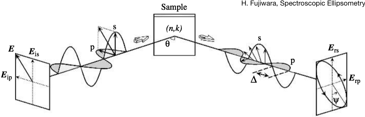
A basic ellipsometer configuration is shown below. Typically the incident light is linearly polarized but the reflected light is, in general, elliptically polarized.
and
The parameter \(\Delta\) describes the change in phase from parallel polarization after reflection (because \(E_p\) and \(E_s\) are in phase before incidence). The amplitude ratio (parallel vs perpendicular reflected light) is represented by \(\tan\psi\).
Fitting to a sinusoid
We want to fit the detected signal \(I(\phi)\) to find average value \(I_\mathrm{DC}\) as well as the two Fourier coefficients \(I_S\) and \(I_C\)
Our ellipsometer digitizes the signal every 5 degrees to produce an array of 72 elements, \(I_i\). The first challenge is to determine the coefficients \(I_\mathrm{DC}\), \(I_S\), and \(I_C\) using these discrete data points
where, \(\phi_i=2\pi i/N\).
The DC offset \(I_\mathrm{DC}\) is found by averaging over one analyzer rotation (\(0\le\phi\le2\pi\))
The Fourier coefficients are given by
For the discrete case this becomes
where \(\Delta\phi=2\pi/N\).
If we substitute for \(\Delta\phi\), then we recognize that \(I_C\) and \(I_S\) are just the weighted averages of \(I_i\) over one drum rotation
where the quantities in brackets need only be calculated once at the beginning of the analysis. Every rotation of the drum requires three averages to be calculated.
Below is a test with random noise added to a known sinusoidal signal.
[2]:
degrees = np.linspace(0, 360, num=72, endpoint=False)
phi = degrees * np.pi / 180

# this is the signal we will try to recover
a = 4.1
b = 0.8
c = 0.5
error = 0.2
signal = ellipse.rotating_analyzer_signal(phi, a, b, c, error)

# finding the offset and coefficients of the sin() and cos() terms
# np.average sums the array and divides by the number of elements N
I_DC = np.average(signal)
I_S = 2 * np.average(signal * np.sin(2 * phi))
I_C = 2 * np.average(signal * np.cos(2 * phi))

plt.scatter(degrees, signal, s=5, color="red")
plt.plot(degrees, I_DC + I_S * np.sin(2 * phi) + I_C * np.cos(2 * phi))
plt.xlabel("Analyzer Angle (degrees)")
plt.ylabel("Ellipsometer Intensity")
plt.xlim(-10, 370)
plt.show()

print("I_DC expected=%.3f obtained=%.3f" % (a, I_DC))
print("I_S  expected=%.3f obtained=%.3f" % (b, I_S))
print("I_C  expected=%.3f obtained=%.3f" % (c, I_C))
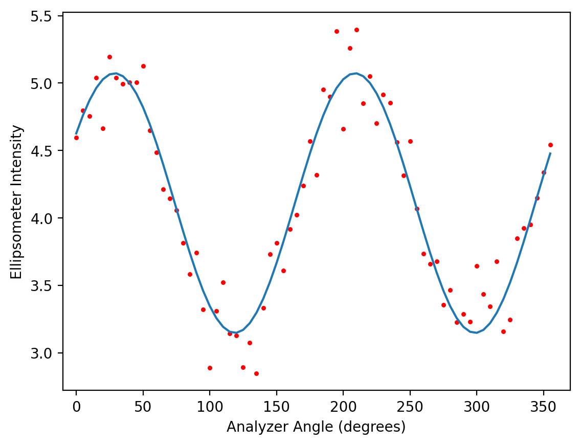
I_DC expected=4.100 obtained=4.110
I_S  expected=0.800 obtained=0.813
I_C  expected=0.500 obtained=0.516
Isotropic, Homogeneous Materials
Converting \(\alpha\) and \(\beta\) to surface properties requires a physical model for the surface. The simplest model is that of an isotropic flat material with reflection determined by the Fresnel reflection properties.
Tompkins 2005, page 282, writes >The major problem with this approach is that it ignores the surface layer of the material. All materials have this surface overlayer, which may due to surface roughness, surface oxide, surface reconstruction, etc. Therefore, any realistic model of the sample is more complicated than a simple air/material, and [this analysis] is not valid for any model involving a surface overlayer. However, [it] is quite useful as a limiting case …
The expression for the electric field at the detector can be found using Jones matrices. The incident light passes through a linear polarizer at an angle \(\theta_p\) relative to the plane of incidence. The light is reflected off the surface and then passes through a linear analyzer at an angle \(\phi\). The electric field is
Therefore
and since the intensity is the product of \(E_D\) with its conjugate transpose \(I=E_D\cdot E_D^\dagger\), with a bit of algebra we find that
and with even more algebra this can be related back to the sinusoidal function
which leads to
[3]:
degrees = np.linspace(0, 360, num=72, endpoint=False)
phi = degrees * np.pi / 180

# create signal
m = 3 - 0.2j  # sample index of refraction
P = 30  # incident polarization azimuth (degrees)
theta_p = np.radians(P)  # incident polarization azimuth (radians)
th = 70  # angle of incidence (degrees)
theta_i = np.radians(th)  # angle of incidence (radians)

# Generate 72 intensities based on experimental conditions
# One reflected intensity for each angle of the rotating analyzer
phi_deg = np.linspace(0, 360, num=72, endpoint=False)
phi = np.radians(phi_deg)
signal = ellipse.rotating_analyzer_signal_from_m(phi, m, theta_i, theta_p, noise=0.003)

# analyze signal
rho, fit = ellipse.rho_from_rotating_analyzer_data(phi, signal, theta_p)
m2 = ellipse.m_from_rho(rho, theta_i)

# display data and fit
plt.plot(degrees, signal, "xr")
plt.plot(degrees, fit)

plt.xlabel("Analyzer Angle (degrees)")
plt.ylabel("Ellipsometer Measurement")
plt.title("%.1f° Linear Polarized Light, No QWP" % np.degrees(theta_p))
plt.xlim(-10, 370)
plt.show()


print("m=%.3f%+.3fj (expected)" % (m.real, m.imag))
print("m=%.3f%+.3fj" % (m2.real, m2.imag))

# rho2 = ellipse.rho_from_m(m,theta_i)
# print("rho=%.3f%+.3fj (expected)"%(rho2.real,rho2.imag))
# print("rho=%.3f%+.3fj"%(rho.real,rho.imag))
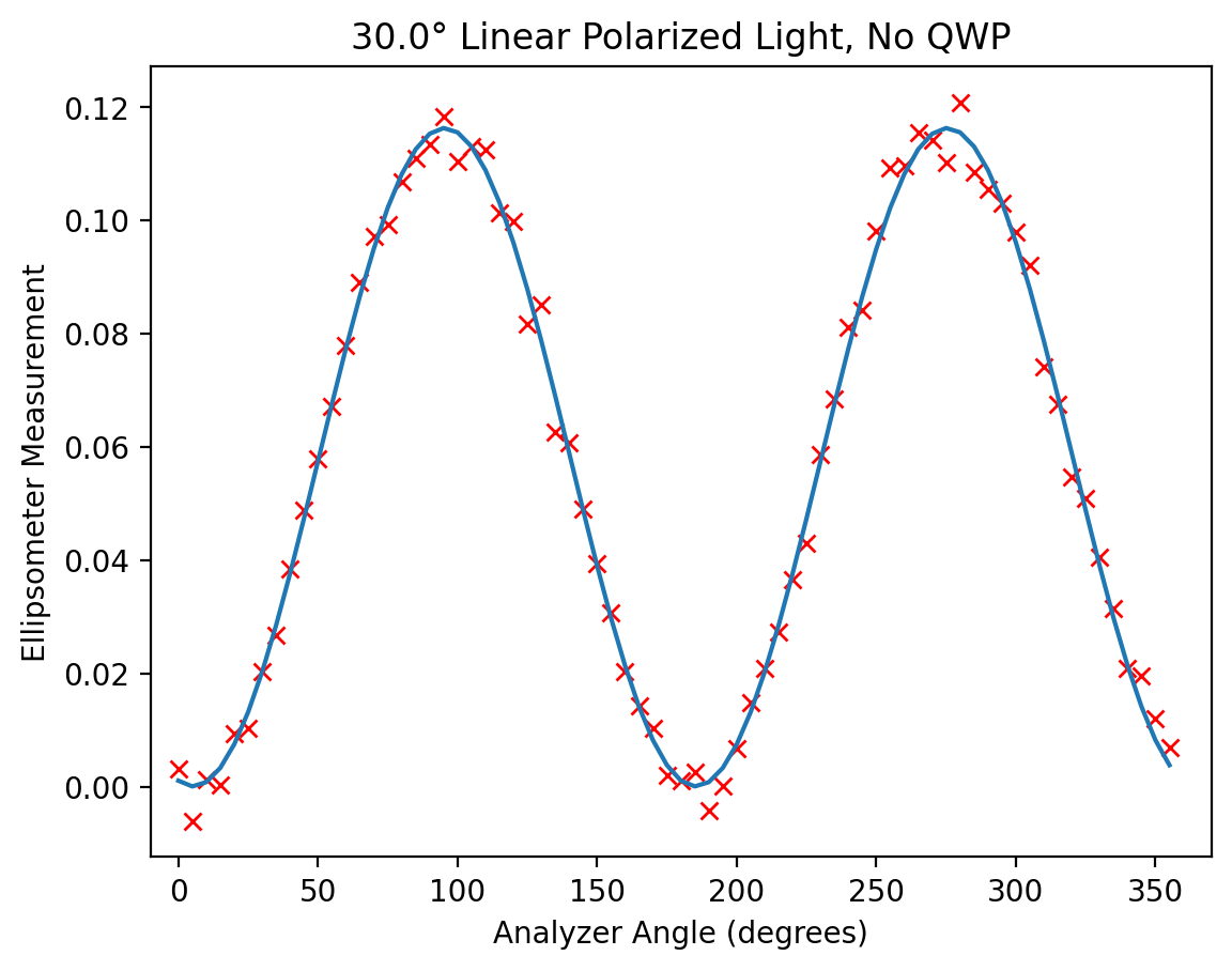
m=3.000-0.200j (expected)
m=3.026-0.047j
Ellipsometry Parameters
If linearly polarized light is incident with an azimuthal angle \(\theta_p\) (where \(\theta_p=0^\circ\) is in the plane of incidence) then the normalized intensity is
No quarter wave plate in the incident beam (\(0\le\theta_p\le90°\))
The parameters \(\psi\) and \(\Delta\) can now be calculated from \(\alpha\) and \(\beta\)
Or in terms of \(I_\mathrm{DC}\), \(I_S\), and \(I_C\)
Example
generate a theoretical ellipsometer signal
fit the signal to determine m
[4]:
# Experimental Conditions
m = 1.5 - 0.0j  # sample index of refraction
P = 45  # incident polarization azimuth (degrees)
theta_p = np.radians(P)  # incident polarization azimuth (radians)
th = 70  # angle of incidence (degrees)
theta_i = np.radians(th)  # angle of incidence (radians)

# Generate 72 intensities based on experimental conditions
# One reflected intensity for each angle of the rotating analyzer
phiD = np.linspace(0, 360, num=72, endpoint=False)
phi = np.radians(phiD)
signal = ellipse.rotating_analyzer_signal_from_m(phi, m, theta_i, theta_p, noise=0.0005)

# Calculate Delta, tanpsi, and index from 72 intensities
rho, fit = ellipse.rho_from_rotating_analyzer_data(phi, signal, theta_p)
m2 = ellipse.m_from_rho(rho, theta_i)
tanpsi, Delta = ellipse.tanpsi_Delta_from_rho(rho)

# Show the results
plt.plot(phiD, signal, "or")
plt.plot(phiD, fit, color="blue")
plt.title(r"P=%d°, $\theta_i=$%d, m=%.1f-%.1fj" % (P, th, m.real, -m.imag))
plt.xlabel("Analyzer Angle (degrees)")
plt.ylabel("Ellipsometer Intensity")
plt.xlim(-10, 370)
plt.show()

print("Fitted Delta=%.1f°, tanpsi=%.3f" % (np.degrees(Delta), tanpsi))
print("Original  refractive index = %.3f%+.3fj" % (m.real, m.imag))
print("Recovered refractive index = %.3f%+.3fj" % (m2.real, m2.imag))
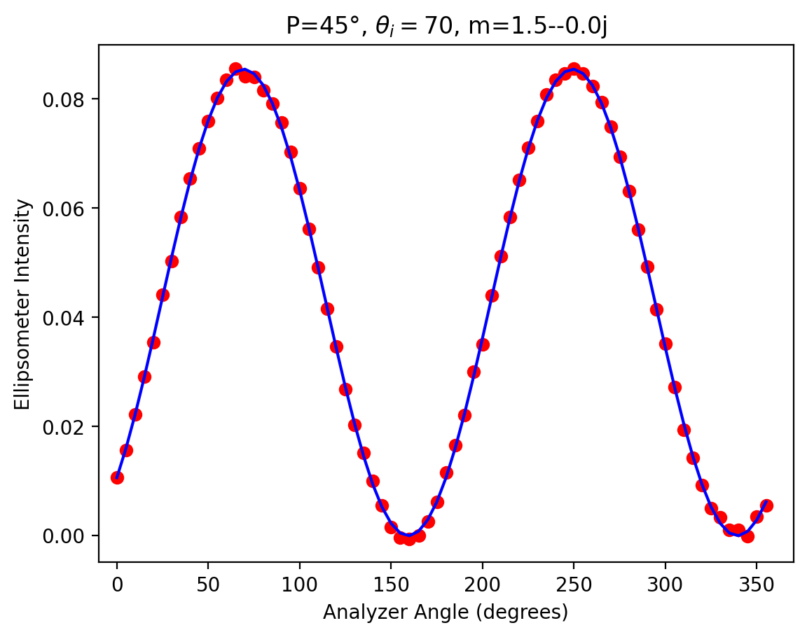
Fitted Delta=0.0°, tanpsi=0.352
Original  refractive index = 1.500+0.000j
Recovered refractive index = 1.554+0.000j
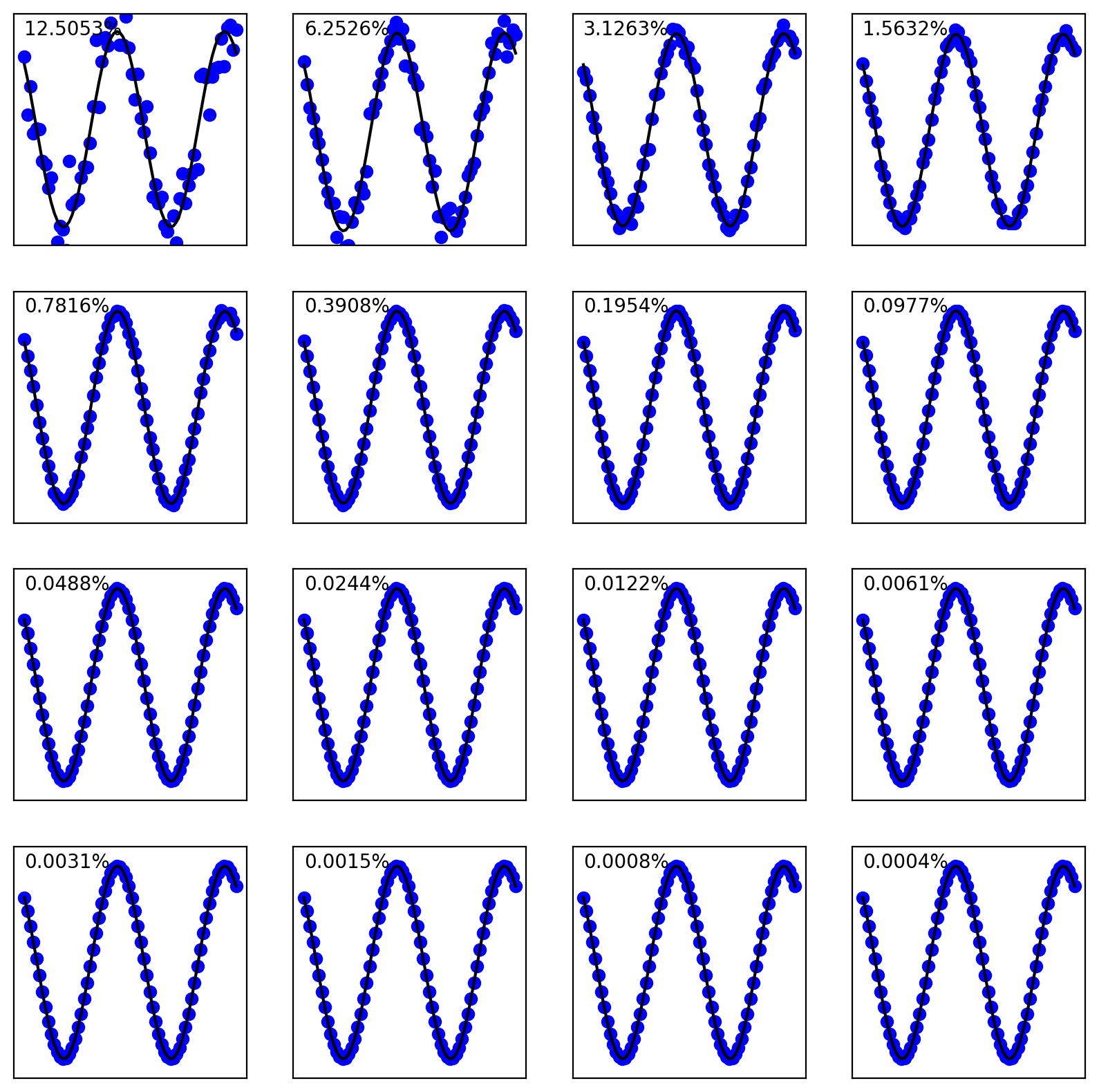
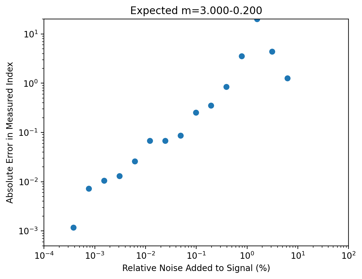
Sensitivity to random Gaussian noise
[5]:
# Experimental Conditions
m = 3.0 - 0.2j  # sample index of refraction
P = 20  # incident linear polarization angle (degrees)
theta_p = np.radians(P)  # incident linear polarization angle (radians)
th = 30  # angle of incidence (degrees)
theta_i = np.radians(th)  # angle of incidence (radians)

# Generate 72 intensities based on experimental conditions
phi = np.radians(np.linspace(0, 360, num=72, endpoint=False))

# error free signal needed to scale the plots
signal = ellipse.rotating_analyzer_signal_from_m(phi, m, theta_i, theta_p)
scale = signal.mean()
ymax = signal.max()

N = 16
dev = np.zeros(N)
err = np.zeros(N)
print("m=%.3f%+.3f  expected" % (m.real, m.imag))

# create fit plots for each error
plt.subplots(4, 4, figsize=(10, 10))
for i in range(N):
    error = scale * 2 ** (-i - 2)
    signal = ellipse.rotating_analyzer_signal_from_m(phi, m, theta_i, theta_p, noise=error)
    rho, fit = ellipse.rho_from_rotating_analyzer_data(phi, signal, theta_p)
    m2 = ellipse.m_from_rho(rho, theta_i)
    dev[i] = abs(m2 - m)
    rel_error = 100 * error / ymax
    err[i] = rel_error
    plt.subplot(4, 4, i + 1)
    plt.plot(np.degrees(phi), signal, "ob")
    plt.plot(np.degrees(phi), fit, "k")
    plt.ylim(-0.1 * ymax, 1.1 * ymax)
    plt.text(0, 0.99 * ymax, "%.4f%%" % rel_error)
    plt.yticks([])
    plt.xticks([])

    print("m=%.3f%+.3f  error=%.3f%%" % (m2.real, m2.imag, rel_error))

plt.show()
plt.scatter(err, dev)
plt.xlim(1e-4, 100)
plt.ylim(5e-4, 20)
plt.xscale("log")
plt.yscale("log")
plt.xlabel("Relative Noise Added to Signal (%)")
plt.ylabel("Absolute Error in Measured Index")
plt.title("Expected m=%.3f%+.3f" % (m.real, m.imag))
plt.show()
m=3.000-0.200  expected
m=118.537+0.000  error=12.505%
m=1.760+0.000  error=6.253%
m=7.396+0.000  error=3.126%
m=23.022+0.000  error=1.563%
m=6.535+0.000  error=0.782%
m=2.649-0.964  error=0.391%
m=3.290+0.000  error=0.195%
m=2.936-0.444  error=0.098%
m=3.010-0.114  error=0.049%
m=2.990-0.267  error=0.024%
m=3.009-0.133  error=0.012%
m=2.996-0.226  error=0.006%
m=2.998-0.213  error=0.003%
m=3.001-0.190  error=0.002%
m=2.999-0.207  error=0.001%
m=3.000-0.201  error=0.000%
Not all measurements give equally good results
[6]:
# Experimental Conditions
phi = np.radians(np.linspace(0, 360, num=72, endpoint=False))
tanpsi = 0.5

print("   P     Delta  tanpsi     Delta  tanpsi  Delta tanpsi")
for P in [1, 45, 89, 91, 178, -10, -89]:
    for Del in [10, 67, 120, 178]:

        Delta = np.radians(Del)
        theta_p = np.radians(P)
        rho0 = tanpsi * np.exp(1j * Delta)

        print("%6.1f° %6.1f° %6.3f:   " % (P, Del, tanpsi), end="")
        #        print(" [%.2f° %.2f] " % (np.degrees(np.angle(rho0)),rho.imag),end='')

        signal = ellipse.rotating_analyzer_signal_from_rho(phi, rho0, theta_p, noise=0.0002)

        rho, fit = ellipse.rho_from_rotating_analyzer_data(phi, signal, theta_p)
        print("%8.3f° %6.3f" % (np.degrees(np.angle(rho)), np.abs(rho)))
   P     Delta  tanpsi     Delta  tanpsi  Delta tanpsi
   1.0°   10.0°  0.500:      1.313°  0.508
   1.0°   67.0°  0.500:     66.879°  0.502
   1.0°  120.0°  0.500:    120.181°  0.503
   1.0°  178.0°  0.500:   -180.000°  0.581
  45.0°   10.0°  0.500:     10.012°  0.500
  45.0°   67.0°  0.500:     67.000°  0.500
  45.0°  120.0°  0.500:    119.998°  0.500
  45.0°  178.0°  0.500:    177.854°  0.500
  89.0°   10.0°  0.500:      0.000°  0.387
  89.0°   67.0°  0.500:     69.778°  0.565
  89.0°  120.0°  0.500:    118.646°  0.520
  89.0°  178.0°  0.500:    156.129°  0.546
  91.0°   10.0°  0.500:     -0.000°  0.668
  91.0°   67.0°  0.500:     64.874°  0.458
  91.0°  120.0°  0.500:    130.141°  0.388
  91.0°  178.0°  0.500:   -180.000°  0.326
 178.0°   10.0°  0.500:     10.102°  0.500
 178.0°   67.0°  0.500:     67.028°  0.499
 178.0°  120.0°  0.500:    120.001°  0.500
 178.0°  178.0°  0.500:    177.165°  0.500
 -10.0°   10.0°  0.500:      9.967°  0.500
 -10.0°   67.0°  0.500:     66.999°  0.500
 -10.0°  120.0°  0.500:    120.004°  0.500
 -10.0°  178.0°  0.500:    178.067°  0.500
 -89.0°   10.0°  0.500:     -0.000°  0.737
 -89.0°   67.0°  0.500:     67.721°  0.516
 -89.0°  120.0°  0.500:    123.377°  0.454
 -89.0°  178.0°  0.500:   -180.000°  0.411
[ ]: