Fresnel Reflectance and Transmittance
Scott Prahl
Feb 2026
[1]:
%config InlineBackend.figure_format = 'retina'

import sys
import numpy as np
import matplotlib.pyplot as plt

if sys.platform == "emscripten":
    import micropip

    await micropip.install("pypolar")

from pypolar import fresnel
Fresnel reflection treats the interaction of plane wave with a flat surface. Usually, Fresnel reflection describes the interaction for a dielectric (e.g., glass), but the equations are sufficiently general that Fresnel reflection can handle semiconductors (e.g., silicon) and metals (e.g., gold) as well.
The general assumption is that the incident light hits the surface at an angle \(\theta\) from the normal and that the surface material is described by an index of refraction coefficient \(m\). The surface must be on an object/layer that is much thicker than the wavelength of light.
This notebook covers the pypolar.fresnel module and is organized
Nomenclature and equation
Complex index of refraction
Example uses
Nomenclature and equations
Plane of incidence
For Fresnel reflectance everything is relative to the plane-of-incidence. This plane is shown below and includes the incoming beam and the normal to the surface. The electric field is decomposed into two parts: the field parallel to the plane of incidence \(E_p\) and the field perpendicular to the plane \(E_s\).
where \(\hat{\mathbf{s}}\) and \(\hat{\mathbf{p}}\) are unit vectors that lie in each plane (and are also perpendicular to the direction of beam propagation).

When an electric plane wave from a vacuum and hits a flat surface at an angle \(\theta\) from the normal to the surface then the reflected electric fields will be
How this affects the beam irradiance requires the Poynting vector which we will get to in a bit!
Fresnel reflectance equations
The Fresnel field reflectances for an angle of incidence \(\theta\) and an index of refraction \(m\) describing the material that the surface is made from is
and
This particular formulation is best for computing because
it works for complex indices of refraction
it works for normal incidence (\(\theta=0\))
it avoids calculating the transmitted angle
Fresnel transmission equations
The Fresnel field transmission coefficients are
and
Fresnel relations for irradiance
Poynting vector and irradiance
The Poynting vector describes the power flux (the energy per unit area per unit time) of an electromagnetic field,
The time-averaged Poynting vector is the irradiance (power/area). For plane waves, this is
where \(I\) is the irradiance and
is the impedance of free space. The factor of 2 arises from time averaging, and the index of refraction \(m\) describes the medium being propagated through.
A note on units. The field \(E\) has units of Volts/meter and so \(\langle \mathbf{S}\rangle\) has units of (Volts/meter)\(^2\)/Ohms. From basic electricity, we know that power \(P=V^2/R\) and so has units of Volts\(^2\) per Ohm. Therefore the time-averaged Poynting vector has units of Watts/meter\(^2\) which is the same as irradiance.
Fresnel relations for irradiance
If the incident irradiance is designated by \(I_0=I_{p0} + I_{s0}\) then the reflected irradiances can be written
or because the irradiance is the square of the electric field
Therefore the reflection coefficients for irradiance are
and
The equations for transmission are a bit trickier because the beam changes cross-sectional area across the boundary
and
Refractive Index
In general, the index of refraction is a complex number
For dielectric materials (glass,water,etc.) the index is real (\(\kappa=0\)
\(\kappa\) represents the absorption of the field by the medium
the sign of imaginary part is negative.
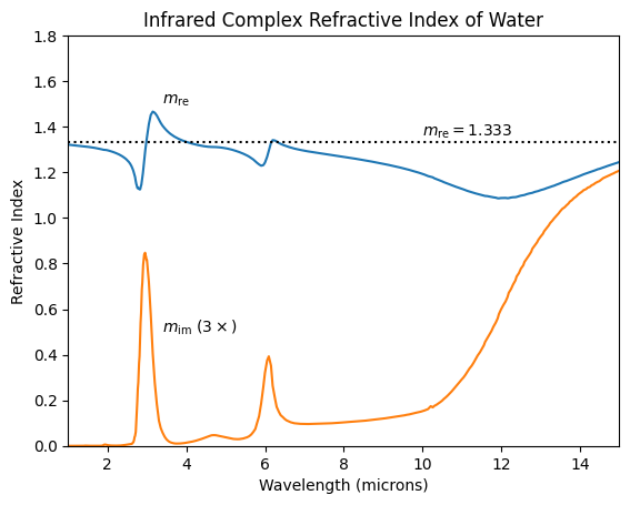
Complex Refractive Index of Water
Let’s import and plot some data from the M.S. Thesis of D. Segelstein, “The Complex Refractive Index of Water”, University of Missouri–Kansas City, (1981) to get some sense the complex index of refraction. The imaginary part shows absorption peaks at 3 and 6 microns, as well as the broad peak starting at 10 microns.
[2]:
# import the Segelstein data
h2o = np.genfromtxt("https://omlc.org/spectra/water/data/segelstein81_index.txt", delimiter="\t", skip_header=4)
h2o_lam = h2o[:, 0]
h2o_mre = h2o[:, 1]
h2o_mim = h2o[:, 2]

# plot it
plt.plot(h2o_lam, h2o_mre)
plt.plot(h2o_lam, h2o_mim * 3)
plt.plot((1, 15), (1.333, 1.333), ":k")
plt.xlim((1, 15))
plt.ylim((0, 1.8))
plt.xlabel("Wavelength (microns)")
plt.ylabel("Refractive Index")
plt.annotate(r"$m_\mathrm{re}$", xy=(3.4, 1.5))
plt.annotate(r"$m_\mathrm{im}\,\,(3\times)$", xy=(3.4, 0.5))
plt.annotate(r"$m_\mathrm{re}=1.333$", xy=(10, 1.36))

plt.title("Infrared Complex Refractive Index of Water")

plt.show()
[3]:
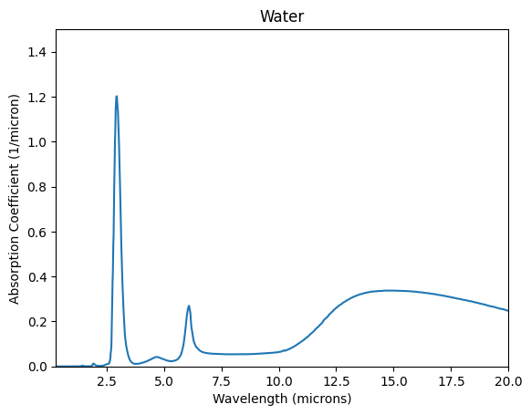
mua = 4 * np.pi * h2o_mim / h2o_lam

plt.plot(h2o_lam, mua)
plt.xlim((0.3, 20))
plt.ylim((0, 1.5))
plt.xlabel("Wavelength (microns)")
plt.ylabel("Absorption Coefficient (1/micron)")

plt.title("Water")

plt.show()
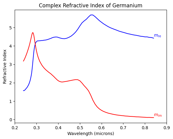
Complex Refractive Index of Germanium
[4]:
# import the Jellison data for germanium
ge = np.genfromtxt(
    "https://refractiveindex.info/tmp/database/data-nk/other/semiconductor%20alloys/Si-Ge/Jellison-11.txt",
    delimiter="\t",
)
# data is stacked so need to rearrange
N = len(ge) // 2
ge_lam = ge[1:N, 0]
ge_mre = ge[1:N, 1]
ge_mim = ge[N + 1 :, 1]

plt.plot(ge_lam, ge_mre, color="blue")
plt.plot(ge_lam, ge_mim, color="red")
plt.xlim((0.2, 0.9))
plt.xlabel("Wavelength (microns)")
plt.ylabel("Refractive Index")
plt.annotate(r"$m_\mathrm{re}$", xy=(ge_lam[-1], ge_mre[-1]), va="bottom", color="blue")
plt.annotate(r"$m_\mathrm{im}$", xy=(ge_lam[-1], ge_mim[-1]), va="bottom", color="red")

plt.title("Complex Refractive Index of Germanium")

plt.show()
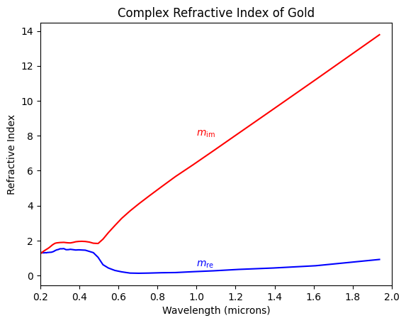
Complex Refractive Index of Gold
[5]:
# import the Johnson and Christy data for gold
au = np.genfromtxt("https://refractiveindex.info/tmp/database/data-nk/main/Au/Johnson.txt", delimiter="\t")

# data is stacked so need to rearrange
N = len(au) // 2
au_lam = au[1:N, 0]
au_mre = au[1:N, 1]
au_mim = au[N + 1 :, 1]

plt.plot(au_lam, au_mre, color="blue")
plt.plot(au_lam, au_mim, color="red")
plt.xlim((0.2, 2))
plt.xlabel("Wavelength (microns)")
plt.ylabel("Refractive Index")
plt.annotate(r"$m_\mathrm{re}$", xy=(1.0, 0.5), color="blue")
plt.annotate(r"$m_\mathrm{im}$", xy=(1.0, 8), color="red")

plt.title("Complex Refractive Index of Gold")

plt.show()
Dielectric Examples
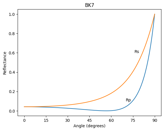
For dielectrics like glass, \(\kappa=0\) and the reflectance as a function of angle looks like The angle at which \(R_p\) goes is a minimum in dielectrics is called Brewster’s angle \(\theta_B\). For semiconductors and metals this angle is called the principal angle of incidence.
[6]:
# BK7
m = complex(1.51508, 0.0)

N = 100
theta = np.linspace(0, 90, N)

Rp = fresnel.R_par(m, theta, deg=True)
Rs = fresnel.R_per(m, theta, deg=True)

plt.plot(theta, Rp)
plt.plot(theta, Rs)
plt.xlabel("Angle (degrees)")
plt.ylabel("Reflectance")
plt.annotate("Rs", xy=(76, 0.6))
plt.annotate("Rp", xy=(70, 0.1))
plt.title("BK7")
plt.xticks([0, 15, 30, 45, 60, 75, 90])


plt.show()
Conservation of field energy at normal incidence
At normal incidence \(\theta=0\),
and
[7]:
rp = fresnel.r_par_amplitude(1.5, 0)
print("At normal incidence r_p=%.3f" % rp)
tp = fresnel.t_par_amplitude(1.5, 0)
print("At normal incidence t_p=%.3f" % tp)
print("tp+rp=%.3f" % (tp + rp))
print()

rs = fresnel.r_per_amplitude(1.5, 0)
print("At normal incidence r_s=%.3f" % rs)
ts = fresnel.t_per_amplitude(1.5, 0)
print("At normal incidence t_s=%.3f" % ts)
print("ts-rs=%.3f" % (ts - rs))
At normal incidence r_p=0.200
At normal incidence t_p=0.800
tp+rp=1.000

At normal incidence r_s=-0.200
At normal incidence t_s=0.800
ts-rs=1.000
Conservation of irradiance at normal incidence
[8]:
Rp = fresnel.R_par(1.5, 0)
print("At normal incidence R_p=%.3f" % Rp)
Tp = fresnel.T_par(1.5, 0)
print("At normal incidence T_p=%.3f" % Tp)
print("Tp+Rp=%.3f" % (Tp + Rp))

print()

Rs = fresnel.R_per(1.5, 0)
print("At normal incidence R_s=%.3f" % Rs)
Ts = fresnel.T_per(1.5, 0)
print("At normal incidence T_s=%.3f" % Ts)
print("Ts+Rs=%.3f" % (Ts + Rs))
At normal incidence R_p=0.040
At normal incidence T_p=0.960
Tp+Rp=1.000

At normal incidence R_s=0.040
At normal incidence T_s=0.960
Ts+Rs=1.000
Conservation at other angles
If m is real, then
but except for \(\theta=0\)
[9]:
m = 1.5
theta = np.linspace(0, 89, 90)

rs = fresnel.r_per_amplitude(m, theta, deg=True)
rp = fresnel.r_par_amplitude(m, theta, deg=True)
ts = fresnel.t_per_amplitude(m, theta, deg=True)
tp = fresnel.t_par_amplitude(m, theta, deg=True)

plt.plot(theta, tp + rp)
plt.plot(theta, ts - rs)

plt.xlabel("Angle of Incidence (degrees)")
plt.ylabel("Combined Reflected and Transmitted Fields")
plt.annotate(r"$t_\bot-r_\bot$", xy=(theta[70], ts[70] - rs[70]), va="top")
plt.annotate(r"$t_\parallel+r_\parallel$  ", xy=(theta[70], tp[70] + rp[70]), ha="right")
plt.title("Refractive Index =%.4f" % m)
plt.xticks([0, 15, 30, 45, 60, 75, 90])


plt.show()
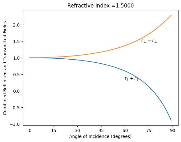
Figure 4.41 in Hecht, Optics, 2002
[10]:
m = 1.5

N = 91
theta = np.linspace(0, 90, N)

rp = fresnel.r_par_amplitude(m, theta, deg=True)
rs = fresnel.r_per_amplitude(m, theta, deg=True)
tp = fresnel.t_par_amplitude(m, theta, deg=True)
ts = fresnel.t_per_amplitude(m, theta, deg=True)

brewster = fresnel.brewster(m, deg=True)

plt.plot(theta, rp)
plt.plot(theta, rs)
plt.plot(theta, tp)
plt.plot(theta, ts)
plt.plot([0, 90], [0, 0], ":k")
plt.plot([brewster, brewster], [-1, 1], ":k")
plt.xlabel("Angle (degrees)")
plt.ylabel("Electric Field Reflectance or Transmittance")
plt.annotate(r"$r_s$", xy=(theta[70], rs[70]))
plt.annotate(r"$r_p$", xy=(theta[70], rp[70]))
plt.annotate(r"$t_s$", xy=(theta[70], 0.85 * ts[70]))
plt.annotate(r"$t_p$", xy=(theta[70], 1.05 * tp[70]))
plt.annotate(r" $\theta_B$", xy=(brewster, 0), va="bottom")

plt.xticks([0, 15, 30, 45, 60, 75, 90])


plt.title("Similar to Hecht figure 4.41 (m=1.5)")

plt.show()
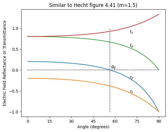
Figure 4.42 in Hecht, Optics, 2002
[11]:
help(fresnel.critical)
Help on function critical in module pypolar.fresnel:

critical(m, n_i=1, deg=False)
    Critical angle for total internal reflection at interface.

    Args:
        m:       complex index of refraction of medium    [-]
        n_i:     real refractive index of incident medium [-]
        deg:     theta_i is in degrees                    [True/False]

    Returns:
        critical angle from normal to surface             [radians/degrees]
[12]:
m = 1.0
n_i = 1.5

critical = fresnel.critical(m, n_i, deg=True)
theta = np.linspace(0, critical, 100)

rp = fresnel.r_par_amplitude(m, theta, n_i, deg=True)
rs = fresnel.r_per_amplitude(m, theta, n_i, deg=True)

plt.plot(theta, rp.real, color="red")
plt.plot(theta, rs.real, color="blue")
plt.plot(theta, rp.imag)

plt.xlabel("Angle (degrees)")
plt.ylabel("Electric Field Reflectance")
plt.text(theta[0], rs[0], r"$r_s$", va="bottom", color="blue")
plt.text(theta[0], rp[0], r"$r_p$", va="bottom", color="red")

plt.title("Similar to Hecht figure 4.42 (m=1/1.5)")

brewster = fresnel.brewster(m, n_i, deg=True)

plt.axvline(brewster, color="black", linestyle=":")
plt.text(brewster, -0.1, r" $\theta_B$", va="bottom")

plt.axvline(critical, color="black", linestyle=":")
plt.text(critical, -0.1, r" $\theta_C$", va="bottom")

plt.axhline(0, color="black")

plt.xticks([0, 15, 30, 45, 60, 75, 90])


plt.show()
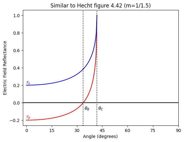
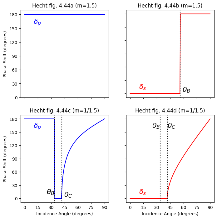
Figure 4.44 in Hecht, Optics, 2002
Now we test the phase shift. This turned out to be a bit tricky, because python was chosing the wrong branch of the sqrt() function. But once that was realized, the graphs match up nicely.
[13]:
N = 181
theta = np.linspace(0, 90, N)
tick_angles = [0, 30, 60, 90, 120, 150, 180]

m = 1.5
n_i = 1.0
rp = fresnel.r_par_amplitude(m, theta, n_i, deg=True)
rs = fresnel.r_per_amplitude(m, theta, n_i, deg=True)
brewster = fresnel.brewster(m, n_i, deg=True)

plt.subplots(2, 2, figsize=(8, 8))

plt.subplot(2, 2, 1)
plt.title("Hecht fig. 4.44a (m=1.5)")
plt.plot(theta, np.angle(rs, deg=True), color="blue")
plt.ylabel("Phase Shift (degrees)")
plt.yticks(tick_angles)
plt.xticks([0, 15, 30, 45, 60, 75, 90])
plt.text(10, 160, r"$\delta_p$", fontsize=16, color="blue")
plt.gca().tick_params(labelbottom=False)

plt.subplot(2, 2, 2)
plt.title("Hecht fig. 4.44b (m=1.5)")
plt.plot(theta, np.angle(rp, deg=True), color="red")
plt.axvline(brewster, color="black", linestyle=":")
plt.yticks(tick_angles)
plt.xticks([0, 15, 30, 45, 60, 75, 90])
plt.text(brewster, -0.0, r" $\theta_B$ ", va="bottom", fontsize=16)
plt.text(10, 10, r"$\delta_s$", fontsize=16, color="red")
plt.gca().tick_params(labelbottom=False, labelleft=False)

m = 1
n_i = 1.5
rs = fresnel.r_per_amplitude(m, theta, n_i, deg=True)
rp = fresnel.r_par_amplitude(m, theta, n_i, deg=True)

brewster = fresnel.brewster(m, n_i, deg=True)
critical = fresnel.critical(m, n_i, deg=True)

plt.subplot(2, 2, 3)
plt.title("Hecht fig. 4.44c (m=1/1.5)")
plt.plot(theta, np.angle(rp, deg=True), color="blue")
plt.axvline(brewster, color="black", linestyle=":")
plt.axvline(critical, color="black", linestyle=":")
plt.xlabel("Incidence Angle (degrees)")
plt.ylabel("Phase Shift (degrees)")
plt.xticks([0, 15, 30, 45, 60, 75, 90])

plt.yticks(tick_angles)
plt.text(brewster, 10, r" $\theta_B$", ha="right", fontsize=16)
plt.text(critical, -0, r" $\theta_C$", va="bottom", fontsize=16)
plt.text(10, 160, r"$\delta_p$", fontsize=16, color="blue")

plt.subplot(2, 2, 4)
plt.plot(theta, np.angle(rs, deg=True), color="red")
plt.xlabel("Incidence Angle (degrees)")
plt.xticks([0, 15, 30, 45, 60, 75, 90])

plt.yticks(tick_angles)
plt.title("Hecht fig. 4.44d (m=1/1.5)")
plt.axvline(brewster, color="black", linestyle=":")
plt.axvline(critical, color="black", linestyle=":")
plt.text(10, 10, r"$\delta_s$", fontsize=16, color="red")
plt.text(brewster, 160, r" $\theta_B$", ha="right", fontsize=16)
plt.text(critical, 160, r"$\theta_C$", fontsize=16)
plt.gca().tick_params(labelleft=False)

plt.show()
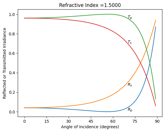
[14]:
m = 1.5
theta = np.linspace(0, 89, 90)

Rs = fresnel.R_per(m, theta, deg=True)
Rp = fresnel.R_par(m, theta, deg=True)
Ts = fresnel.T_per(m, theta, deg=True)
Tp = fresnel.T_par(m, theta, deg=True)

plt.plot(theta, Rp)
plt.plot(theta, Rs)
plt.plot(theta, Tp)
plt.plot(theta, Ts)

plt.xlabel("Angle of Incidence (degrees)")
plt.ylabel("Reflected or Transmitted Irradiance")
plt.annotate(r"$R_s$", xy=(theta[70], Rs[70]), va="top")
plt.annotate(r"$R_p$", xy=(theta[70], Rp[70]), va="top")
plt.annotate(r"$T_s$", xy=(theta[70], Ts[70]))
plt.annotate(r"$T_p$", xy=(theta[70], Tp[70]))
plt.title("Refractive Index =%.4f" % m)
plt.xticks([0, 15, 30, 45, 60, 75, 90])


plt.show()
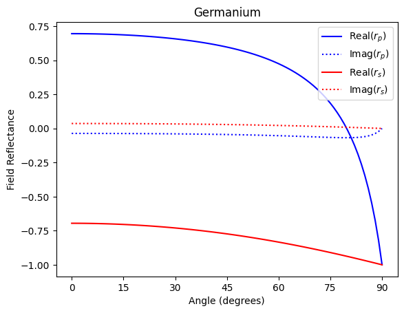
Semiconductor Examples
For semi-conductors like germanium (\(m=5.47392- j 0.771829\) at \(\lambda\)=633nm) the reflectance as a function of angle looks like
[15]:
# Germanium
m = complex(5.47392, -0.771829)

N = 91
theta = np.linspace(0, 90, N)

rp = fresnel.r_par_amplitude(m, theta, deg=True)
rs = fresnel.r_per_amplitude(m, theta, deg=True)

plt.plot(theta, rp.real, "b", label=r"Real($r_p$)")
plt.plot(theta, rp.imag, "b:", label=r"Imag$(r_p)$")
plt.plot(theta, rs.real, "r", label=r"Real$(r_s)$")
plt.plot(theta, rs.imag, "r:", label=r"Imag$(r_s)$")
plt.xlabel("Angle (degrees)")
plt.ylabel("Field Reflectance")
plt.xticks([0, 15, 30, 45, 60, 75, 90])
# plt.annotate('Rs',  xy=(76, 0.8))
# plt.annotate('Rp',  xy=(70, 0.13))
plt.title("Germanium")
plt.legend()

plt.show()
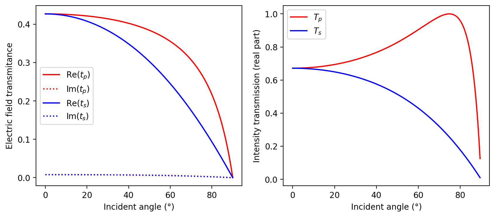
[16]:
# From https://refractiveindex.info/?shelf=main&book=GaAs&page=Aspnes, for 0.8 um = 800 nm

ref_index = 3.6835 - 0.085660j
theta = np.linspace(0, 90, 181)

tp = fresnel.t_par_amplitude(ref_index, theta, deg=True)
ts = fresnel.t_per_amplitude(ref_index, theta, deg=True)

Tp = fresnel.T_par(ref_index, theta, deg=True)
Ts = fresnel.T_per(ref_index, theta, deg=True)

plt.figure(figsize=(10, 4))
plt.subplot(1, 2, 1)
plt.plot(theta, tp.real, "r", label=r"Re($t_p$)")
plt.plot(theta, tp.imag, ":r", label=r"Im($t_p$)")
plt.plot(theta, ts.real, "b", label=r"Re($t_s$)")
plt.plot(theta, ts.imag, ":b", label=r"Im($t_s$)")
plt.ylabel("Electric field transmitance")
plt.xlabel("Incident angle (°)")
plt.legend()

plt.subplot(1, 2, 2)
plt.plot(theta[:-1], Tp.real[:-1], "r", label="$T_p$")
plt.plot(theta[:-1], Ts.real[:-1], "b", label="$T_s$")
plt.ylabel("Intensity transmission (real part)")
plt.xlabel("Incident angle (°)")
plt.legend()

plt.show()
Metal Examples
Gold
For metals like gold the index of refraction is \(m=0.176717 - j 3.03779\) at \(\lambda\)=633nm. Note that the minimum in \(R_p\) is much larger than zero and is called the principal polarization angle.
[17]:
# Gold
m = complex(0.176717, -3.03779)

N = 91
theta = np.linspace(0, 90, N)

Rp = fresnel.R_par(m, theta, deg=True)
Rs = fresnel.R_per(m, theta, deg=True)

plt.plot(theta, Rp)
plt.plot(theta, Rs)
plt.xlabel("Angle (degrees)")
plt.ylabel("Reflectance")
plt.title("Gold")
plt.annotate("Rs", xy=(76, 0.98))
plt.annotate("Rp", xy=(70, 0.89))
plt.xticks([0, 15, 30, 45, 60, 75, 90])


plt.show()

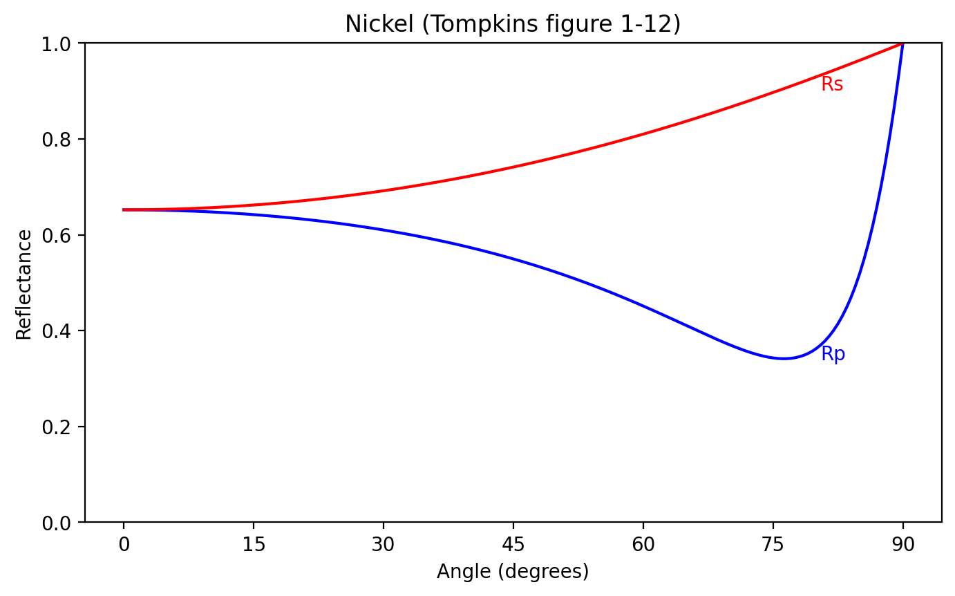
Nickel
See Tompkins, A User’s Guide to Ellipsometry, 1993, figure 1-12 on page 44.
[18]:
# Nickel
m = complex(2.01, -3.75)

N = 181
theta = np.linspace(0, 90, N)

Rp = fresnel.R_par(m, theta, deg=True)
Rs = fresnel.R_per(m, theta, deg=True)

plt.plot(theta, Rp, color="blue")
plt.plot(theta, Rs, color="red")
plt.xlabel("Angle (degrees)")
plt.ylabel("Reflectance")
plt.annotate("Rs", xy=(theta[-20], Rs[-20]), color="red", va="top")
plt.annotate("Rp", xy=(theta[-20], Rp[-20]), color="blue", va="top")
plt.title("Nickel (Tompkins figure 1-12)")
plt.ylim(0, 1)
plt.xticks([0, 15, 30, 45, 60, 75, 90])


plt.show()
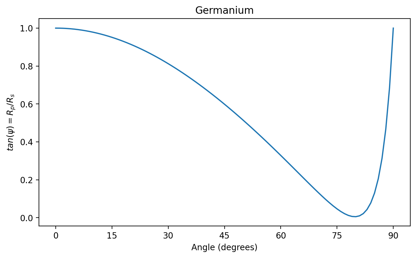
Ellipsometry graphs
\(\tan\psi\)
One important parameter used in ellipsometry is the ratio of the parallel and perpendicular reflected light. This is commonly expressed as \(\tan\psi\) is defined as
This non-dimensional parameter allows simple measurements of surfaces that give information about things like
Film thickness
Refractive Index (\(n\))
Extinction Coefficient (\(\kappa\))
Surface Roughness Anisotropy
Retardation
Phase Difference
Birefringence
[19]:
# Germanium
m = complex(5.47392, -0.771829)

N = 91
theta = np.linspace(0, 90, N)
th = np.radians(theta)
tanpsi = fresnel.R_par(m, theta, deg=True) / fresnel.R_per(m, theta, deg=True)

plt.plot(theta, tanpsi)
plt.xlabel("Angle (degrees)")
plt.ylabel("$tan(\psi)=R_p/R_s$")
plt.title("Germanium")
plt.xticks([0, 15, 30, 45, 60, 75, 90])


plt.show()
Behavior at 45°
Finally at 45\(^\circ\) the square of the perpendicular reflectance equals the parallel reflectance
[20]:
# Silver
m = complex(0.0574411, -4.27996)

N = 100
theta = np.linspace(0, 90, N)

Rp = fresnel.R_par(m, theta, deg=True)
Rs = fresnel.R_per(m, theta, deg=True) ** 2

plt.plot(theta, Rp)
plt.plot(theta, Rs)
plt.plot([45, 45], [0.97, 1.00], ":k")
plt.xticks([0, 15, 30, 45, 60, 75, 90])
plt.xlabel("Angle (degrees)")
plt.ylabel("Reflectance")
plt.title("Silver")
plt.annotate("$R_s^2$", xy=(76, 0.997))
plt.annotate("$R_p$", xy=(70, 0.975))
plt.xticks([0, 15, 30, 45, 60, 75, 90])


plt.show()

[ ]: