Jones Calculus Examples
Scott Prahl
Feb 2026
Basic examples and visualization options for the pypolar.jones module.
This module and many optics texts (including Fowles) define angles based on the receiver point-of-view. This means that the electric field is viewed against the direction of propagation or on looking into the source. Complete details of the conventions used can be found in this Jupyter notebook on Conventions
[1]:
%config InlineBackend.figure_format = 'retina'

import sys
import numpy as np
import matplotlib.pyplot as plt

if sys.platform == "emscripten":
    import micropip

    await micropip.install("pypolar")

from pypolar import jones
from pypolar import visualization as vis
Optical isolator
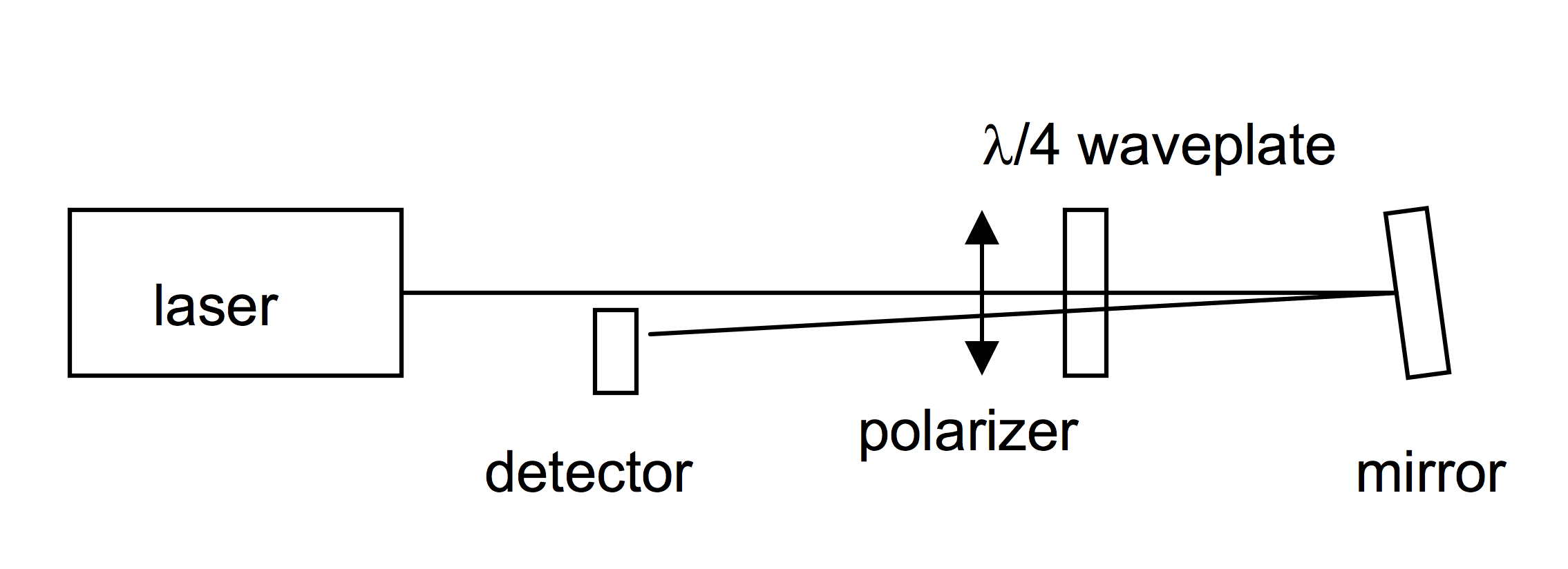
The path through the system is (b) linear polarizer at lab angle 0°, (C) QWP at 45°, (D) mirror , (E) QWP from the opposite side so -45°, linear polarizer at 0°
[2]:
B = jones.op_linear_polarizer(0)
C = jones.op_quarter_wave_plate(np.pi / 4)
D = jones.op_mirror()
E = jones.op_quarter_wave_plate(-np.pi / 4)
F = jones.op_linear_polarizer(0)
We can find the operator for these elements by multiplying all the matrices together. This is done using the @ operator (since python 3.5).
He we find the overall polarization operator for the five polarization elements is the zero matrix! Therefore any incident polarization state will be zeroed out — exactly what is needed for an optical isolator.
[3]:
W = F @ E @ D @ C @ B
print(np.round(W, 3))
[[0.+0.j 0.+0.j]
 [0.+0.j 0.+0.j]]
It is worth emphasizing that @ is required. The usual * operator only multiplies elements together and therefore ends up with the wrong result!
[4]:
W = F * E * D * C * B
print(np.round(W, 3))
[[0.5+0.j 0. +0.j]
 [0. +0.j 0. +0.j]]
Compare C @ D with D * C and it is clear that the two methods give completely different results.
[5]:
print(np.round(C @ D, 3))
print()
print(np.round(C * D, 3))
[[ 0.707+0.j     0.   -0.707j]
 [ 0.   +0.707j -0.707+0.j   ]]

[[ 0.707+0.j  0.   +0.j]
 [ 0.   +0.j -0.707+0.j]]
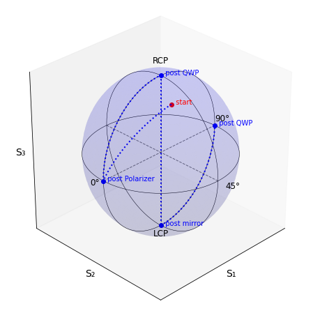
Visualization on Poincaré Sphere
Start with an arbitrary elliptical polarization state and see how by the second pass the polarization state is always linearly polarized at 90°.
[6]:
fig = plt.figure(figsize=(8, 8))
ax = fig.add_subplot(111, projection="3d")
vis.draw_empty_sphere(ax)

# J1 = jones.field_elliptical(np.random.random()*np.pi,np.random.random()*2*np.pi)

J1 = jones.field_elliptical(np.pi / 6, np.pi / 6)

J2 = B @ J1
J3 = C @ J2
J4 = D @ J3
J5 = E @ J4

vis.draw_jones_poincare(J1, ax, label="  start", color="red", va="center")
vis.draw_jones_poincare(J2, ax, label="  after Polarizer", color="blue", va="center")
vis.draw_jones_poincare(J3, ax, label="  after QWP", color="blue", va="center")
vis.draw_jones_poincare(J4, ax, label="  after mirror", color="blue", va="center")
vis.draw_jones_poincare(J5, ax, label="  final", color="red", va="center")

vis.join_jones_poincare(J1, J2, ax, color="blue", lw=2, linestyle=":")
vis.join_jones_poincare(J2, J3, ax, color="blue", lw=2, linestyle=":")
vis.join_jones_poincare(J3, J4, ax, color="blue", lw=2, linestyle=":")
vis.join_jones_poincare(J4, J5, ax, color="blue", lw=2, linestyle=":")
plt.show()
[ ]: