Null Ellipsometry

Scott Prahl

April 2020

Null ellipsometry determines $\psi$ and $\Delta$ by rotating the polarizer and analyzer to extinction. This notebook reviews zone conventions, predicts expected settings for BK7 and crystalline silicon at 632.8nm, and compares those predictions with measured null angles.

References

Archer, Manual on Ellipsometry 1968.
Azzam, Ellipsometry and Polarized Light, 1977.
Fujiwara, Spectroscopic Ellipsometry, 2007.
McCrackin, “Measurement of the Thickness and Refractive Index of Very Thin Films and the Optical Properties of Surfaces by Ellipsometry,” J. of the National Bureau of Standards, 67A, 363–377, 1963.
Tompkins, A User’s Guide to Ellipsometry, 1993
Tompkins, Handbook of Ellipsometry, 2005.
Woollam, A Short Course in Ellipsometry, 2001.

[1]:

%config InlineBackend.figure_format = 'retina'

import sys
import numpy as np
import matplotlib.pyplot as plt

if sys.platform == "emscripten":
    import micropip

    await micropip.install("pypolar")

from pypolar import fresnel
from pypolar import jones
from pypolar import visualization as vis
from pypolar import ellipsometry as ellipse

m_bk7 = 1.5151  # index of BK7 at 632.8nm
m_si = 3.875 - 0.023j  # index of crystalline silicon at 632.8nm

Overview

Layout

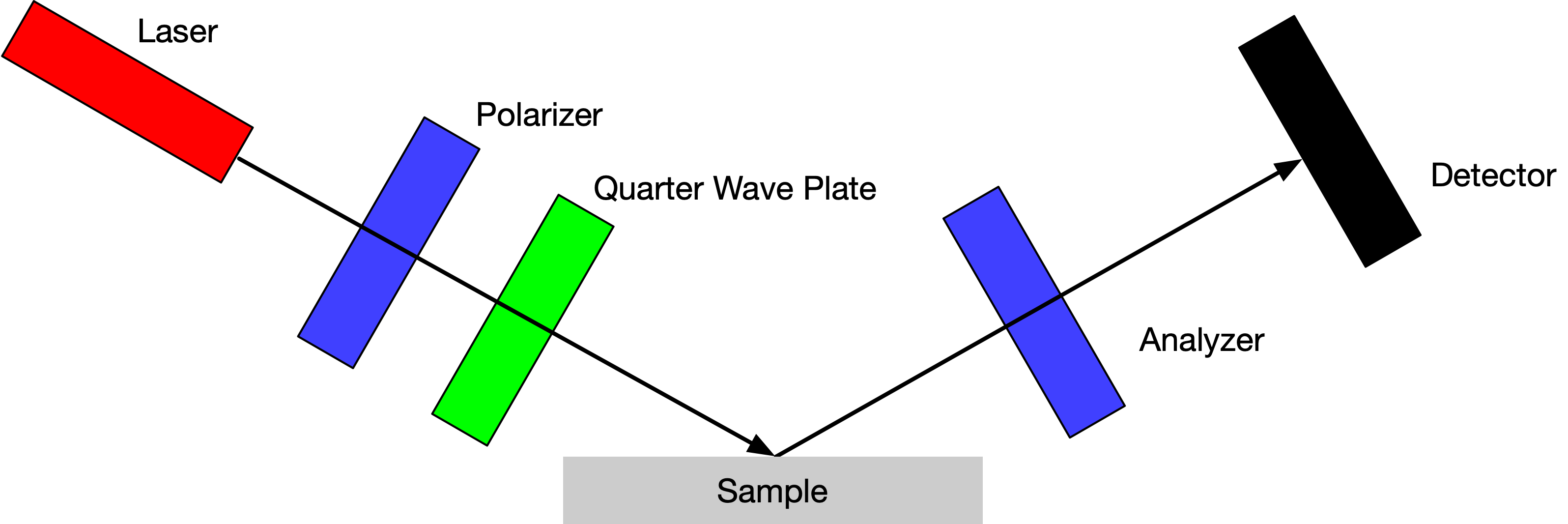
caaaae2ea1fb4e438c9369744a30875b

A typical layout for a null ellipsometer is shown above. An unpolarized (or circularly polarized) laser beam is incident on a linear polarizer set at an angle $\theta_p$. The light then passes through a quarter wave plate (QWP) set at ±45° to the plane of incidence. The light emerging from the polarizer will in general be elliptically polarized. This light hits the sample and the reflected light passes through an analyzer (at $\theta_a$) before reaching the detector.

In null ellipsometry, the polarizer and analyzer are rotated until no light reaches the detector. These angles are used to determine $\tan\psi$ and $\Delta$, which in turn, are used to calculate the complex refractive index of the sample.

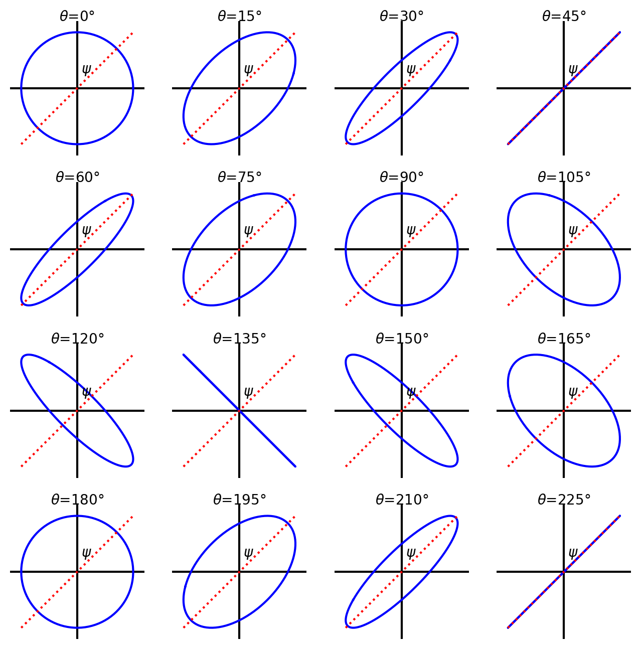
It is not immediately obvious that the combination of a linear polarizer and quarter-wave plate can produce an arbitrary elliptical polarization state. The figure below shows different polarization states as the linear polarizer is rotated relative to the QWP.

[2]:

qwp = jones.op_quarter_wave_plate(np.pi / 4)

plt.subplots(4, 4, figsize=(8, 8))
for i in range(16):
    plt.subplot(4, 4, i + 1)
    th = 15 * i
    theta = np.radians(th)
    pol = jones.field_linear(theta)
    result = qwp @ pol
    vis.draw_jones_ellipse(result, simple=True)
    plt.xticks([])
    plt.yticks([])
    plt.text(0, 0.85, r"$\theta$=%d°" % th, ha="center")

Ellipsometry Zones

McCrackin summarizes

For any given surface there is a multiplicity of polarizer, analyzer, and compensator scale settings that produce extinction by the analyzer of the reflected light from the surface, and it becomes somewhat of a problem to determine the values of $\Delta$ and $\psi$ from these various readings. In order to explain how these numerous readings arise and how $\Delta$ and $\psi$ may be computed from them it is well to keep two facts in mind: (a) all azimuthal angles are measured positive counter-clockwise from the plane of incidence when looking into the light beam, and

the compensator, which may be set at any azimuth, is generally set so that its fast axis is in an azimuth of $\pm\pi/4$…

The various readings fall into four sets called zones, two with the fast axis of the compensator set at $\pi/4$, numbered 2 and 4, and two with it set at $-\pi/4$, numbered 1 and 3. In each zone there is one independent set of polarizer and analyzer readings, making four independent sets of $\theta_p$ and $\theta_a$ readings in all. However, since both analyzer and polarizer may be rotated by $\pi$ without affecting the results, there are 16 polarizer and analyzer settings falling into four independent zones. Since the compensator may also be rotated by $\pi$ without affecting the results, there are 32 possible sets of readings on the ellipsometer.

The various null angles fall into four sets called zones, two with the fast-axis of the quarter wave plate set 45° (2 & 4) and two with the fast-axis of the quarter wave plate set to -45° (1 & 3). In each zone there are four combinations of polarizer and analyzer angles that have a null reading (because rotating a linear polarizer by 180° gives the same result). Identifying the right values to determine $\psi$ and $\Delta$ is still confusing, so McCrackin introduces three new parameters ($p$, $a_s$, and $a_p$) to simplify

Rather than calculating $\Delta$ and $\psi$ directly from the $\theta_p$ and $\theta_a$ values, it is useful to calculate three other quantities, $p$, $a_p$, and $a_s$, from the $\theta_p$ and $\theta_a$ values, $p$ being related to the $\theta_p$ readings, $a_p$, related to the $\theta_a$ readings in zones 1 and 4, and $a_s$, related to the $\theta_a$ readings in zones 2 and 3. For a perfect quarterwave plate these are related to $\Delta$ and $\psi$ by

Zone	QWP Orientation	Polarizer Angle $\theta_p$	Analyzer Angle $\theta_a$
1	$-\pi/4$	$p$	$a_p$
		$p+\pi$	$a_p$
		$p$	$a_p+\pi$
		$p+\pi$	$a_p+\pi$

3	$-\pi/4$	$p+ \pi/2$	$ \pi-a_s$
		$p+3\pi/2$	$ \pi-a_s$
		$p+ \pi/2$	$2\pi-a_s$
		$p+3\pi/2$	$2\pi-a_s$

2	$+\pi/4$	$ \pi/2-p$	$a_s$
		$3\pi/2-p$	$a_s$
		$ \pi/2-p$	$a_s+\pi$
		$3\pi/2-p$	$a_s+\pi$

4	$+\pi/4$	$ \pi-p$	$ \pi-a_p$
		$2\pi-p$	$ \pi-a_p$
		$ \pi-p$	$2\pi-a_p$
		$2\pi-p$	$2\pi-a_p$

So for an ellipsometer with the QWP at 45°, there are eight different polarizer/analyzer pairs that will null the reflected light. The $\psi$ and $\Delta$ values are readily calculated from these using:

\[\Delta = \frac{\pi}{2} +2p \qquad\mbox{and}\qquad \psi=a_s = a_p\]

When the QWP is oriented 45° to the plane of incidence then zones 2 and 4 are of interest. Of the four possible polarizer/analyzer pairs, the first entry for zone 2 and the last entry in zone 4 can be used.

We know that $0\le\psi\le\pi/2$ and that $0\le\Delta\le2\pi$ and use these to derive constraints for range of polarizer and analyzer angles for each zone. These are shown graphically below.

[3]:

plt.figure(figsize=(8, 4.5))
plt.xlim(-180, 180)
plt.ylim(-180, 180)
plt.xticks([-180, -135, -90, -45, 0, 45, 90, 135, 180])
plt.yticks([-180, -90, 0, 90, 180])

plt.axhspan(0, 90, 3 / 8, 7 / 8, color="pink")
plt.text(45, 45, "Zone 2", fontsize=20, ha="center", va="center")

plt.axhspan(0, -90, 1 / 8, 5 / 8, color="lightblue")
plt.text(-45, -45, "Zone 4", fontsize=20, ha="center", va="center")

plt.xlabel("Polarizer Setting")
plt.ylabel("Analyzer Setting")
plt.title("Quarter Wave Plate at 45°")
plt.grid(True)

plt.show()

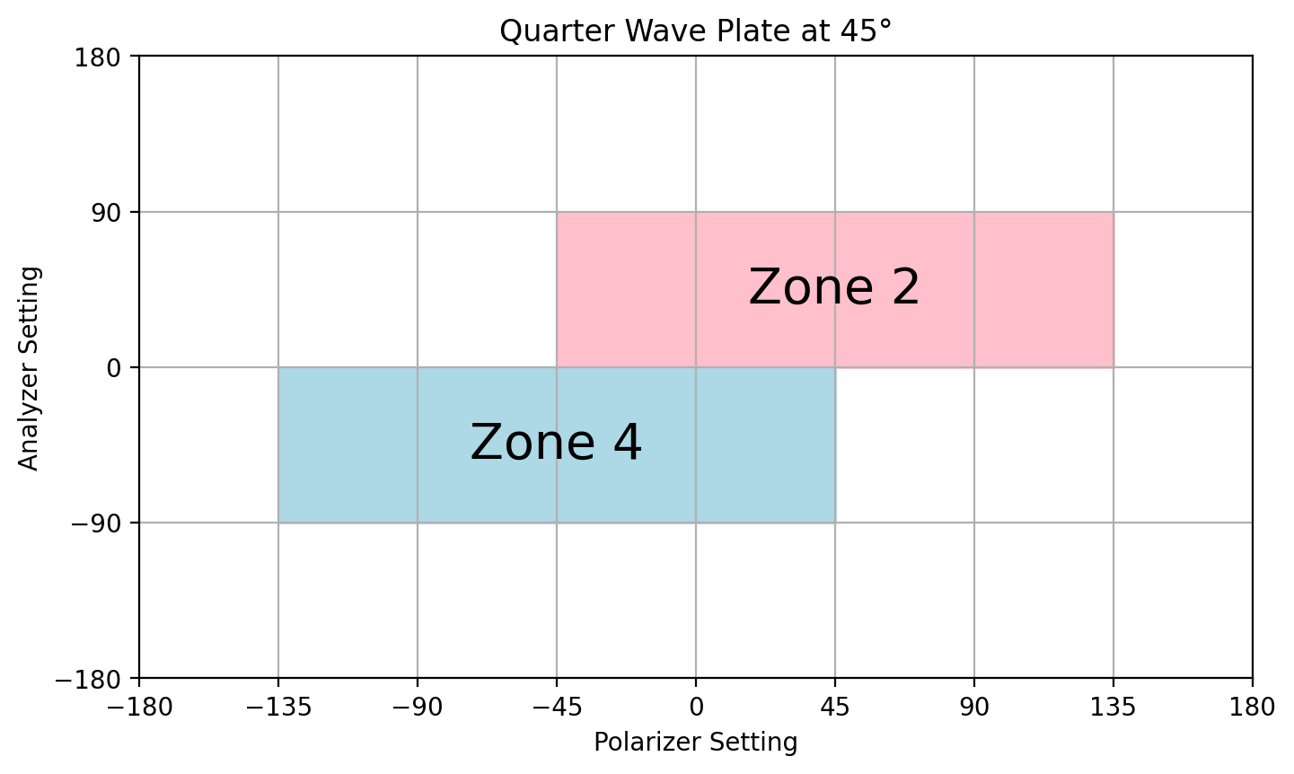
Zone 2

We know that $0\le\psi\le\pi/2$ and that $0\le\Delta\le2\pi$. Therefore with a bit of algebra, the first row of zone 2 leads to the requirement that the analyzer must be between 0° and 90°:

\[0°<\theta_{a2}<90° \quad\mbox{and}\quad -45°<\theta_{p2}\le135°\]

when both conditions are satisfied, then

\[\psi = \theta_{a2} \quad\mbox{and}\quad \Delta = 270°-2\theta_{p2}\]

Notice that when $\theta_{p2}=135°$ then $\Delta=0$; this means that the index of refraction has no imaginary part and is a real number.

Zone 4

For zone 4, the last row in Table 1 requires the analyzer to be between -90° and 0°

\[-90°<\theta_{a4}<0° \quad\mbox{and}\quad -135°<\theta_{p4}\le45°\]

when both conditions are satisfied, then

\[\psi = -\theta_{a4} \quad\mbox{and}\quad \Delta = 90°-2\theta_{p4}\]

Now when $\theta_{p4}=45°$ then $\Delta=0$; this means that the index of refraction is again purely real.

Averaging results

Since $\psi$ and $\Delta$ are the same for both zones this means that

\[\theta_{a2} = - \theta_{a4} \qquad\mbox{and}\qquad \theta_{p2} = 90° + \theta_{p4}\]

McCrackin showed that averaging $\psi$ and $\Delta$ from zones 2 and 4 should eliminate errors due to inexact compensation by the QWP.

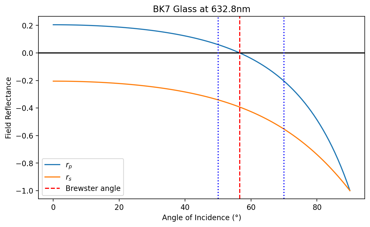
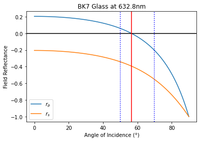
BK7

Consider incidence angles both less than and greater than the Brewster’s angle. We see that the phase change for angles below Brewster’s angle has $\Delta=180°$ and we have $\exp(-j \pi)=-1$ and there is a sign change in the Fresnel reflection, but the overall index of refraction remains real.

Above Brewster’s angle $\Delta=0°$ and the Fresnel reflection is positive and real. In the figure below Brewster’s angle is shown in red. The two dotted blue lines are the fixed ellipsometer incidence angles of 50° and 70°.

[4]:

angle = np.linspace(0, 90, 100)
brew = np.degrees(np.arctan(m_bk7))

rp = fresnel.r_par_amplitude(m_bk7, np.radians(angle))
rs = fresnel.r_per_amplitude(m_bk7, np.radians(angle))

plt.figure(figsize=(8, 4.5))
plt.plot(angle, rp, label="$r_p$")
plt.plot(angle, rs, label="$r_s$")
plt.axhline(0, color="black")
plt.axvline(50, color="blue", linestyle=":")
plt.axvline(70, color="blue", linestyle=":")
plt.axvline(brew, color="red", linestyle="--", label="Brewster angle")


plt.xlabel("Angle of Incidence (°)")
plt.ylabel("Field Reflectance")
plt.title("BK7 Glass at 632.8nm")
plt.legend()
plt.show()

[5]:

plt.figure(figsize=(8, 4.5))
plt.plot(angle, np.degrees(np.arctan(np.abs(rp / rs))), label="arctan($r_p/r_s$)")
plt.axvline(50, color="blue", linestyle=":")
plt.axvline(70, color="blue", linestyle=":")

plt.xlabel("Angle of Incidence (°)")
plt.ylabel(R"$\psi$ (degrees)")
plt.title("BK7 Glass at 632.8nm")
plt.legend()
plt.show()

[6]:

plt.figure(figsize=(8, 4.5))
plt.plot(angle, np.degrees(np.angle(rs) - np.angle(rp)), label=r"$\Delta=\arg(r_s)-\arg(r_p)$")
plt.axvline(50, color="blue", linestyle=":")
plt.axvline(70, color="blue", linestyle=":")

plt.xlabel("Angle of Incidence (°)")
plt.ylabel("Phase of Reflectance")
plt.title("BK7 Glass at 632.8nm")
plt.legend()
plt.show()

Expected angles

[7]:

theta_i = np.radians(50)
s = ellipse.null_angles_report(m_bk7, theta_i)
print(s)

m       = 1.5151+0.0000j
theta_i =    50.0°

zone  P   theta_a
  1      0.8°      0.2°
  1      3.9°      0.2°
  1      0.8°      3.3°
  1      3.9°      3.1°

  3      2.4°      3.0°
  3      5.5°      3.0°
  3      2.4°      6.1°
  3      5.5°      6.1°

  2      0.8°      0.2°
  2      3.9°      0.2°
  2      0.8°      3.3°
  2      3.9°      3.3°

  4      2.4°      3.0°
  4      5.5°      3.0°
  4      2.4°      6.1°
  4      5.5°      6.1°

p       =    45.0°
a       =    10.1°

psi     =    10.1°
Delta   =   180.0°

[8]:

theta_i = np.radians(70)
s = ellipse.null_angles_report(m_bk7, theta_i)
print(s)

m       = 1.5151+0.0000j
theta_i =    70.0°

zone  P   theta_a
  1      5.5°      0.4°
  1      2.4°      0.4°
  1      5.5°      3.5°
  1      2.4°      3.1°

  3      0.8°      2.8°
  3      3.9°      2.8°
  3      0.8°      5.9°
  3      3.9°      5.9°

  2      2.4°      0.4°
  2      5.5°      0.4°
  2      2.4°      3.5°
  2      5.5°      3.5°

  4      3.9°      2.8°
  4      0.8°      2.8°
  4      3.9°      5.9°
  4      0.8°      5.9°

p       =   -45.0°
a       =    20.3°

psi     =    20.3°
Delta   =     0.0°

Measured angles

These measured P2/A2/P4/A4 values are manual null readings entered directly from instrument scale settings for this example dataset.

[9]:

theta_i = np.radians(50)
P2 = np.radians(45)
A2 = np.radians(9.5)
rho2 = ellipse.rho_from_zone_2_null_angles(P2, A2)
m2 = ellipse.m_from_rho(rho2, theta_i)

P4 = np.radians(315.0 - 360)
A4 = np.radians(348.7 - 360)
rho4 = ellipse.rho_from_zone_4_null_angles(P4, A4)
m4 = ellipse.m_from_rho(rho4, theta_i)
m = (m2 + m4) / 2

print("Incidence   = %6.1f°" % np.degrees(theta_i))
print("Measured P2 = %6.1f°" % np.degrees(P2))
print("Measured A2 = %6.1f°" % np.degrees(A2))
print("Measured P4 = %6.1f°" % np.degrees(P4))
print("Measured A4 = %6.1f°" % np.degrees(A4))
print()
print("Derived index of refraction")
print("%.3f%+.3fj (zone 2)" % (m2.real, m2.imag))
print("%.3f%+.3fj (zone 4)" % (m4.real, m4.imag))
print("%.3f%+.3fj (average)" % (m.real, m.imag))

Incidence   =   50.0°
Measured P2 =   45.0°
Measured A2 =    9.5°
Measured P4 =  -45.0°
Measured A4 =  -11.3°

Derived index of refraction
1.492-0.000j (zone 2)
1.569-0.000j (zone 4)
1.530-0.000j (average)

[10]:

theta_i = np.radians(70)
P2 = np.radians(135)
A2 = np.radians(19)
rho2 = ellipse.rho_from_zone_2_null_angles(P2, A2)
m2 = ellipse.m_from_rho(rho2, theta_i)

P4 = np.radians(45)
A4 = np.radians(-20.1)
rho4 = ellipse.rho_from_zone_4_null_angles(P4, A4)
m4 = ellipse.m_from_rho(rho4, theta_i)

print("Incidence   = %6.1f°" % np.degrees(theta_i))
print("Measured P2 = %6.1f°" % np.degrees(P2))
print("Measured A2 = %6.1f°" % np.degrees(A2))
print("Measured P4 = %6.1f°" % np.degrees(P4))
print("Measured A4 = %6.1f°" % np.degrees(A4))
print()
print("Derived index of refraction")
print("%.3f%+.3fj (zone 2)" % (m2.real, m2.imag))
print("%.3f%+.3fj (zone 4)" % (m4.real, m4.imag))
print("%.3f%+.3fj (average)" % (m.real, m.imag))

Incidence   =   70.0°
Measured P2 =  135.0°
Measured A2 =   19.0°
Measured P4 =   45.0°
Measured A4 =  -20.1°

Derived index of refraction
1.571+0.000j (zone 2)
1.523+0.000j (zone 4)
1.530-0.000j (average)

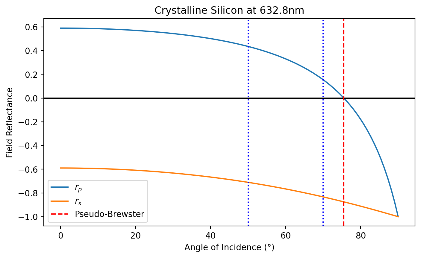
Crystalline Silicon

Crystalline silicon is absorbing at 632.8nm, so there is no true Brewster angle. The red dashed line in the first plot marks the pseudo-Brewster angle (the minimum of $|r_p|$).

[11]:

angle = np.linspace(0, 90, 100)
rp = fresnel.r_par_amplitude(m_si, np.radians(angle))
rs = fresnel.r_per_amplitude(m_si, np.radians(angle))
pseudo_brew = angle[np.argmin(np.abs(rp))]

plt.figure(figsize=(8, 4.5))
plt.plot(angle, rp.real, label="$r_p$")
plt.plot(angle, rs.real, label="$r_s$")
plt.axhline(0, color="black")
plt.axvline(50, color="blue", linestyle=":")
plt.axvline(70, color="blue", linestyle=":")
plt.axvline(pseudo_brew, color="red", linestyle="--", label="Pseudo-Brewster")


plt.xlabel("Angle of Incidence (°)")
plt.ylabel("Field Reflectance")
plt.title("Crystalline Silicon at 632.8nm")
plt.legend()
plt.show()

[12]:

plt.figure(figsize=(8, 4.5))
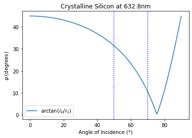
plt.plot(angle, np.degrees(np.arctan(np.abs(rp / rs))), label="arctan($r_p/r_s$)")
plt.axvline(50, color="blue", linestyle=":")
plt.axvline(70, color="blue", linestyle=":")

plt.xlabel("Angle of Incidence (°)")
plt.ylabel(R"$\psi$ (degrees)")
plt.title("Crystalline Silicon at 632.8nm")

plt.legend()
plt.show()

[13]:

plt.figure(figsize=(8, 4.5))
plt.plot(angle, np.degrees(np.angle(rs) - np.angle(rp)), label=r"$\Delta=\arg(r_s)-\arg(r_p)$")
plt.axvline(50, color="blue", linestyle=":")
plt.axvline(70, color="blue", linestyle=":")

plt.xlabel("Angle of Incidence (°)")
plt.ylabel("Phase of Reflectance")
plt.title("Crystalline Silicon at 632.8nm")

plt.legend()
plt.show()

Expected angles

[14]:

theta_i = np.radians(50)
s = ellipse.null_angles_report(m_si, theta_i)
print("****Crystalline Silicon****\n\n", s)

****Crystalline Silicon****

 m       = 3.8750-0.0230j
theta_i =    50.0°

zone  P   theta_a
  1      0.8°      0.5°
  1      3.9°      0.5°
  1      0.8°      3.7°
  1      3.9°      3.1°

  3      2.4°      2.6°
  3      5.5°      2.6°
  3      2.4°      5.7°
  3      5.5°      5.7°

  2      0.8°      0.5°
  2      3.9°      0.5°
  2      0.8°      3.7°
  2      3.9°      3.7°

  4      2.4°      2.6°
  4      5.5°      2.6°
  4      2.4°      5.7°
  4      5.5°      5.7°

p       =    44.9°
a       =    31.5°

psi     =    31.5°
Delta   =   179.8°

[15]:

theta_i = np.radians(70)
s = ellipse.null_angles_report(m_si, theta_i)
print("****Crystalline Silicon****\n\n", s)

****Crystalline Silicon****

 m       = 3.8750-0.0230j
theta_i =    70.0°

zone  P   theta_a
  1      0.8°      0.2°
  1      3.9°      0.2°
  1      0.8°      3.3°
  1      3.9°      3.1°

  3      2.3°      3.0°
  3      5.5°      3.0°
  3      2.3°      6.1°
  3      5.5°      6.1°

  2      0.8°      0.2°
  2      3.9°      0.2°
  2      0.8°      3.3°
  2      3.9°      3.3°

  4      2.4°      3.0°
  4      5.5°      3.0°
  4      2.4°      6.1°
  4      5.5°      6.1°

p       =    44.5°
a       =    10.5°

psi     =    10.5°
Delta   =   179.1°

Measured angles

These measured P2/A2/P4/A4 values are manual null readings entered directly from instrument scale settings for this example dataset.

[16]:

theta_i = np.radians(50)
P2 = np.radians(42.2)
A2 = np.radians(32.1)
rho2 = ellipse.rho_from_zone_2_null_angles(P2, A2)
m2 = ellipse.m_from_rho(rho2, theta_i)

P4 = np.radians(316.5 - 360)
A4 = np.radians(328.5 - 360)
rho4 = ellipse.rho_from_zone_4_null_angles(P4, A4)
m4 = ellipse.m_from_rho(rho4, theta_i)
m = (m2 + m4) / 2

print("Incidence   = %6.1f°" % np.degrees(theta_i))
print("Measured P2 = %6.1f°" % np.degrees(P2))
print("Measured A2 = %6.1f°" % np.degrees(A2))
print("Measured P4 = %6.1f°" % np.degrees(P4))
print("Measured A4 = %6.1f°" % np.degrees(A4))
print()
print("Derived index of refraction")
print("%.3f%+.3fj (zone 2)" % (m2.real, m2.imag))
print("%.3f%+.3fj (zone 4)" % (m4.real, m4.imag))
print("%.3f%+.3fj (average)" % (m.real, m.imag))

Incidence   =   50.0°
Measured P2 =   42.2°
Measured A2 =   32.1°
Measured P4 =  -43.5°
Measured A4 =  -31.5°

Derived index of refraction
3.895-0.757j (zone 2)
3.837-0.379j (zone 4)
3.866-0.568j (average)

[17]:

theta_i = np.radians(70)
P2 = np.radians(55.8)
A2 = np.radians(10.4)
rho2 = ellipse.rho_from_zone_2_null_angles(P2, A2)
m2 = ellipse.m_from_rho(rho2, theta_i)

P4 = np.radians(-34.2)
A4 = np.radians(-10.9)
rho4 = ellipse.rho_from_zone_4_null_angles(P4, A4)
m4 = ellipse.m_from_rho(rho4, theta_i)
m = (m2 + m4) / 2

print("Incidence   = %6.1f°" % np.degrees(theta_i))
print("Measured P2 = %6.1f°" % np.degrees(P2))
print("Measured A2 = %6.1f°" % np.degrees(A2))
print("Measured P4 = %6.1f°" % np.degrees(P4))
print("Measured A4 = %6.1f°" % np.degrees(A4))
print()
print("Derived index of refraction")
print("%.3f%+.3fj (zone 2)" % (m2.real, m2.imag))
print("%.3f%+.3fj (zone 4)" % (m4.real, m4.imag))
print("%.3f%+.3fj (average)" % (m.real, m.imag))

Incidence   =   70.0°
Measured P2 =   55.8°
Measured A2 =   10.4°
Measured P4 =  -34.2°
Measured A4 =  -10.9°

Derived index of refraction
3.722-0.488j (zone 2)
3.778-0.522j (zone 4)
3.750-0.505j (average)

[ ]:

Zone	QWP Orientation	Polarizer Angle \(\theta_p\)	Analyzer Angle \(\theta_a\)
1	\(-\pi/4\)	\(p\)	\(a_p\)
		\(p+\pi\)	\(a_p\)
		\(p\)	\(a_p+\pi\)
		\(p+\pi\)	\(a_p+\pi\)

3	\(-\pi/4\)	\(p+ \pi/2\)	$ \pi-a_s$
		\(p+3\pi/2\)	$ \pi-a_s$
		\(p+ \pi/2\)	\(2\pi-a_s\)
		\(p+3\pi/2\)	\(2\pi-a_s\)

2	\(+\pi/4\)	$ \pi/2-p$	\(a_s\)
		\(3\pi/2-p\)	\(a_s\)
		$ \pi/2-p$	\(a_s+\pi\)
		\(3\pi/2-p\)	\(a_s+\pi\)

4	\(+\pi/4\)	$ \pi-p$	$ \pi-a_p$
		\(2\pi-p\)	$ \pi-a_p$
		$ \pi-p$	\(2\pi-a_p\)
		\(2\pi-p\)	\(2\pi-a_p\)