Polarization & Ellipses
Scott Prahl
Feb 2026
[1]:
%config InlineBackend.figure_format = 'retina'

import sys
import numpy as np
import matplotlib.pyplot as plt

plt.rcParams["animation.html"] = "jshtml"

if sys.platform == "emscripten":
    import micropip

    await micropip.install("pypolar")

from pypolar import jones
from pypolar import visualization as vis

np.set_printoptions(suppress=True)  # print 1e-16 as zero
Introduction
Polarized light in its most general form is called elliptical because when the electric field is projected onto the \(z = 0\) plane it will trace out an ellipse. This projection is called a sectional pattern.
The generally accepted convention is that one views the sectional plane by looking along the \(z\)-axis towards the source. Complete details of the assumptions can be found in Jupyter notebook on Conventions
This notebook examines this ellipse. An ellipse is characterized by its semi-major axis \(a\) and its semi-minor axis \(b\). If the ellipse is not tilted, then the semi-major axis coincides with the \(x\)-axis and therefore \(a=E_{x0}\) and \(b=E_{y0}\).
When the ellipse is rotated at an angle \(\alpha\) from the \(x\)-axis this angle is called the azimuth of the ellipse.
The ellipticity of the ellipse is just \(b/a\). The ellipticity angle is \(\beta\) and is related to the ellipticity by \(b/a=\tan\beta\).
Another angle of interest is the related to the ratio of the field amplitudes \(E_{0y}/E_{0x} = \tan\epsilon\).
[2]:
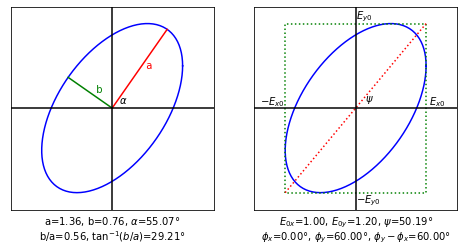
phi = np.pi / 3
v = np.array([1, 1.2 * np.exp(phi * 1j)])
vis.draw_jones_ellipse(v)
plt.show()
[3]:
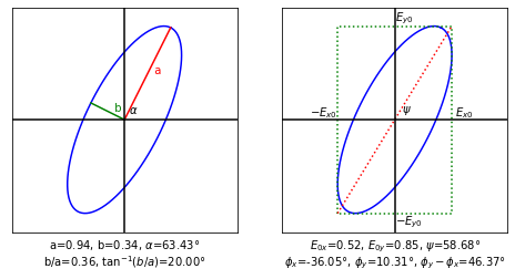
v = jones.field_elliptical(np.arctan(2), np.radians(20))
vis.draw_jones_ellipse(v)
plt.show()
[4]:
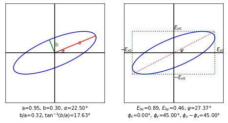
v = 0.325 * np.array([2.732, 1 + 1j])
vis.draw_jones_ellipse(v)
plt.show()
[5]:
v = jones.field_left_circular()

psi = jones.amplitude_ratio_angle(v)
alpha = jones.ellipse_azimuth(v)
beta = jones.ellipticity_angle(v)
a, b = jones.ellipse_axes(v)
E_x, E_y = np.abs(v)
phase = jones.phase(v)

vis.draw_jones_ellipse(v)
plt.show()

print("Jones vector for left circular polarization")
print("    ", v)
print()
print("        pypolar expected")

print("E_x0    %6.3f   %6.3f" % (E_x, 1 / np.sqrt(2)))
print("E_y0    %6.3f   %6.3f" % (E_y, 1 / np.sqrt(2)))
print("psi     %6.1f°  %6.2f° arctan(Ey0/Ex0)" % (np.degrees(psi), 45))
print("phase   %6.2f°  %6.2f° relative" % (np.degrees(phase), -90))
print()

print("alpha   %6.1f°  %6.1f° angle of the semi-major-axis" % (np.degrees(alpha), 45))
print("a       %6.3f   %6.3f semi-major" % (a, 1 / np.sqrt(2)))
print("b       %6.3f   %6.3f semi-minor" % (b, 1 / np.sqrt(2)))
print("b/a     %6.2f   %6.2f" % (b / a, 1.0))
print("beta    %6.1f°  %6.1f° ellipticity arctan(b/a)" % (np.degrees(beta), -45))
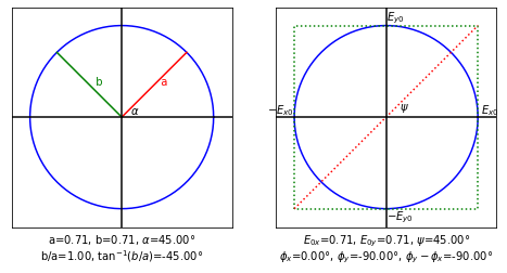
Jones vector for left circular polarization
     [0.70710678+0.j         0.        -0.70710678j]

        pypolar expected
E_x0     0.707    0.707
E_y0     0.707    0.707
psi       45.0°   45.00° arctan(Ey0/Ex0)
phase   -90.00°  -90.00° relative

alpha     45.0°    45.0° angle of the semi-major-axis
a        0.707    0.707 semi-major
b        0.707    0.707 semi-minor
b/a       1.00     1.00
beta     -45.0°   -45.0° ellipticity arctan(b/a)
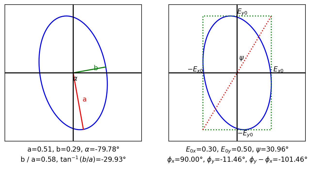
Example from Shurcliff 1964, page 28
[6]:
v = np.array([0.3 * np.exp(1j * np.pi / 2), 0.5 * np.exp(-0.2j)])

gamma = jones.phase(v)
psi = jones.amplitude_ratio_angle(v)
alpha = jones.ellipse_azimuth(v)
beta = jones.ellipticity_angle(v)
a, b = jones.ellipse_axes(v)
E_x, E_y = np.abs(v)

vis.draw_jones_ellipse(v)
plt.show()

print("Jones vector")
print("    ", v)
print()
print("         pypolar Shurcliff")

print("E_x0      %6.1f   %6.1f" % (E_x, 0.3))
print("E_y0      %6.1f   %6.1f" % (E_y, 0.5))
print("psi       %6.1f°  %6.1f° arctan(Ey0/Ex0)" % (np.degrees(psi), 59))
print("gamma     %6.1f°  %6.1f° phase difference (phi_y-phi_x)" % (np.degrees(gamma), -101))
print()
print("alpha     %6.1f°  %6.1f° auxilary angle to major-axis" % (np.degrees(alpha), 10 - 90))
print("alpha+90° %6.1f°  %6.1f° auxilary angle to minor-axis" % (90 + np.degrees(alpha), 10))
print("b/a       %6.2f   %6.2f (semi-minor radius)/(semi-major radius)" % (b / a, 0.58))
print("beta      %6.1f°  %6.1f° ellipticity arctan(b/a)" % (np.degrees(beta), -30))
Jones vector
     [1.83697020e-17+0.3j        4.90033289e-01-0.09933467j]

         pypolar Shurcliff
E_x0         0.3      0.3
E_y0         0.5      0.5
psi         59.0°    59.0° arctan(Ey0/Ex0)
gamma     -101.5°  -101.0° phase difference (phi_y-phi_x)

alpha      -79.8°   -80.0° auxilary angle to major-axis
alpha+90°   10.2°    10.0° auxilary angle to minor-axis
b/a         0.58     0.58 (semi-minor radius)/(semi-major radius)
beta       -29.9°   -30.0° ellipticity arctan(b/a)
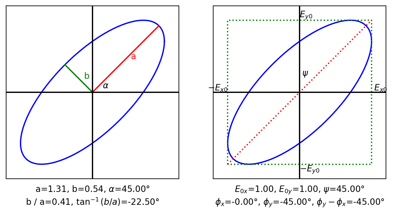
Problem 5.19 and 5.20 from Hecht, Schuam’s Outline of Optics, 1975
Hecht uses \(\exp(kz-\omega t)\) and therefore we need to use the alternate convention. A quick visualization confirms that the E-field rotates counter-clockwise and agres with Hecht that the field is left-handed.
[7]:
jones.use_alternate_convention(True)

v = np.array([1.0, 1.0 * np.exp(1j * np.pi / 4.0)])

vis.draw_jones_ellipse(v)
plt.show()

ani = vis.draw_jones_animated(v, nframes=32)

# The rest of the parameters in Hecht

Delta = jones.phase(v)
psi = jones.amplitude_ratio_angle(v)
alpha = jones.ellipse_azimuth(v)
beta = jones.ellipticity_angle(v)
a, b = jones.ellipse_axes(v)
E_x, E_y = np.abs(v)

jones.use_alternate_convention(False)

print("Jones vector")
print("    ", v)
print()
print("            pypolar   Hecht")

print("alpha        %6.1f°  %6.1f°  horizontal to major-axis" % (np.degrees(alpha), 45))
print("a            %6.3f   %6.3f  semi-major axis" % (a, 1.31))
print("b            %6.3f   %6.3f  semi-minor axis" % (b, 0.542))
print("b/a          %6.2f   %6.2f  " % (b / a, 0.41))
print("ellipticity  %6.1f°  %6.1f°  arctan(b/a)" % (np.degrees(beta), 22.5))

print()
print("E_x0         %6.1f   %6.1f" % (E_x, 1))
print("E_y0         %6.1f   %6.1f" % (E_y, 1))
print("psi          %6.1f°  %6.1f°  arctan(Ey0/Ex0)" % (np.degrees(psi), 45))
print("phi_y-phi_x  %6.1f°  %6.1f° " % (np.degrees(Delta), 45))

ani
Jones vector
     [1.        +0.j         0.70710678+0.70710678j]

            pypolar   Hecht
alpha          45.0°    45.0°  horizontal to major-axis
a             1.307    1.310  semi-major axis
b             0.541    0.542  semi-minor axis
b/a            0.41     0.41
ellipticity    22.5°    22.5°  arctan(b/a)

E_x0            1.0      1.0
E_y0            1.0      1.0
psi            45.0°    45.0°  arctan(Ey0/Ex0)
phi_y-phi_x    45.0°    45.0°
[7]:
[ ]: